Lab 8: Spectral Signature Analysis & Resource Monitoring

Goals and Background

The goal of this lab is to gain the knowledge necessary to measure and interpret spectral reflectance signatures of various surface, and near surface features of the Earth using satellite imagery. Spectral signature curves are used to help analysts to identify, classify, and map land surface features as well as to determine which bands should be used to differentiate features with similar spectral signatures.  Another section of this lab provides experience with some basic Earth resource monitoring functions available in Erdas Imagine. Vegetation density can be monitored using normalized difference vegetation index (NDVI), which ratios reflectance of the red and near infrared bands from Landsat TM, ETM+, or OLI. Another operation can be run to analyze distribution of ferrous mineral in the soil by ratioing the reflectance levels of the middle and near infrared bands.  

Methods

In part one of this lab; spectral signatures are made by creating an area of interest within the feature to be analyzed and using the supervised raster function, signature editor. This process is done for twelve different surface and near surface features found in a Landsat ETM+ image of Eau Claire and surrounding areas. Each signature is then separately analyzed for the bands exhibiting the highest and lowest levels of reflectance and the characteristics of vegetation and soils of different moisture levels analyzed.  The signatures are then all plotted together and analyzed to find bands with the best separability. In the second part of this lab, two different band ratio functions are performed for the purpose of resource monitoring in an image of Eau Claire and Chippewa counties. The processes use unsupervised raster functions to produce an image depicting vegetation density and another depicting the distribution of ferrous mineral content in exposed soil. Both of these images are then brought into Arc map and made into interval classification maps with five classifications in each to better display the information provided in each.

Results

This lab emphasizes the importance of a basic understanding of the interactions of the electromagnetic spectrum with various surface features is an important component in analyzing spectral signatures. It also provides a small look at the broad range of applications in the field of spectral signature analysis. 

Spectral signatures vary between surfaces, but tend to be similar between sub-classifications of surfaces, such as different soil types. Moisture level of the surface feature effects its spectral signature and can be used to differentiate between similar surfaces, as can be observed when the spectral signature of wet and dry soil are plotted together (figure 1). Plotting all spectral signatures together (figure 2) is helpful for the determination of the best bands for separability of signatures. 

Resource monitoring functions in Erdas Imagine produce images helpful in analyzing the resource being monitored, however Arc map has functions that allow the variations to be more clear (figures 3 and 4).

Figure 1. Spectral signatures of wet and dry soils

Figure 2. Spectral signatures of all surfaces analyzed

Figure 3. Vegetation abundance map
produced using NDVI image

Figure 4. Ferrous mineral map

Sources

Satellite image is from Earth Resources Observation and Science Center, United States Geological Survey. 

Background information is from Analyzing Spectral Signature lecture slides, Cyril Wilson, 2016 

Lab 7: Photogrammetry

Goals and Background

Photogrammetry is the process of using pictures to make real world measurements. Its most common application has been in topographic mapping but in more recent years has been applied to wide range of fields such as; architecture, engineering, bathymetries, geology, and many more (Pillai). This lab is designed to provide experience with some of the primary photogrammetric tasks. The tasks included in this lab are calculation of photographic scale, measurement of area and perimeter of a surface, and the calculation of relief displacement. The lab also provides an introduction to stereoscopy to add the illusion of depth to an image and orthorectification to planimetrically correct an image.

Methods

Part 1: Scales, measurements and relief displacement

Section one of this part of the lab begins with the calculation of scale from some given information. The first scenario includes a photograph with two marked points and the real world distance between those points are provided. The image distance then needs to be measured and scale can be calculated by converting the ground distance from feet to inches, plugging the values into the equation S= photo distance/ground distance, then setting this ration equal to 1/X to find the correct ratio for the scale. The second scenario provides the camera`s focal length, the altitude the photograph the photo was taken at, and the elevation of the city below. In this case scale is found using the equation S= focal length/(altitude-elevation), where altitude is altitude above sea level and elevation is of the terrain. Section two introduces the ‘Measure Perimeters and Areas’ digitizing tool in Erdas Imagine. A lagoon in the photograph is digitized and upon completion information is given about perimeter and area of the polygon that was digitized. The unit of each measurement can be easily changed using a drop down menu; in this area is reported in hectares and acres and the perimeter is reported in meters and miles. The third and final section of this part deals with calculation of relief displacement in an image. The image`s scale is provided as well as the height the aerial camera was at above datum when the photograph was taken. The equation used to solve this problem is D= (hxr)/H; where h is the real world height of the object, r is the radial distance from the top of the displaced object to the principal point of the photo, and H is the height of the camera above local datum. The type of adjustment necessary can be determined by this value, a positive value indicates the object must be plotted inward and a negative value indicates it must be plotted outward. 

Part 2: Stereoscopy

In this part of the lab three dimensional images are created using elevation models. In the first section an anaglyph is created by superimposing a digital elevation model (DEM) over a high resolution satellite image of the same area. When viewed wearing polaroid glasses, the resulting image displays areas of higher elevation in three dimension. In the second section of this lab an anaglyph is created of the same area only this time a digital surface model (DSM) is superimposed over the high resolution image. The resulting anaglyph includes many more three dimensional areas due to the fact that a DSM includes elevation information about all objects on the surface and the DEM only includes information about the surface itself.

Part 3: Orthorectification

In this part of the lab Erdas Imagine Lecia Photogrammetric Suite (LPS) is used to provide experience with digital photogrammetry, specifically triangulation and orthorectification. The tasks involved in the production of an orthophoto using two previously orthorecitfied images as references include; creating a new project, selecting a horizontal reference source, collecting GCP`s, adding a second image to the block file, and collecting GCPs in the second image. The LPS Project Manager is found in the toolbox, once opened a new block file is created, setting the appropriate geometric model and horizontal reference projection. The first reference image and the image to be rectified are then added to the project. Nine GCPs are then collected; X and Y values of target locations for each GCP are given for accuracy assessment. Two additional GCPs are collected in the same manner, from a different horizontal reference image. Now a digital elevation model is set as a vertical reference source, once it has been set the Z values for all the collected GCPs can be gathered by simply selecting them all and clicking the Update Z values on Selected Points. In the next section of this part the second reference image is added and GCPs are collected according to the coordinates of GCPs previously created, excluding reference points not located on the original image. The next step is to collect automatic tie points, perform triangulation, and ortho resample the image. Tie points are points found in the areas of overlap between the images, their coordinates are unknown but are found during triangulation. The LPS conveniently places these and the accuracy can be checked after the process of collection is complete. The triangulation process can then be run to find the tie point`s coordinates based off the known GCP coordinates. A report is produced by the triangulation process that includes coordinate and other information. The ortho resampling process is now run and the result can be viewed in the project manager (figure 1) as well as in an Imagine viewer (figure 2).

Results

This lab provided a lot of useful experience with photogrammetric processes. Image scale is a required component of photogrammetry as is the understanding of the various equations that can be used to calculate it from different know information. Knowledge of image displacement and correction of it is also an important photogrammetric concept. An orthophoto can be used to measure many things, including perimeters and areas of objects and surfaces. This lab provided knowledge of how to do that using Erdas Imagine. Stereoscopy can be used to enhance the perception of elevation in an image, as seen from the production of anaglyphs using a DEM and a DSM. Finally, the orthorectification is very long and very tedious, but it is the key to producing an orthophoto usable in photogrammetry applications.

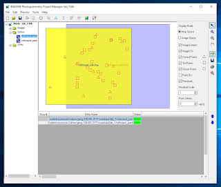Figure 1. Completed orthorectification in Project Manager

Figure 2. Orthophoto displayed in Erdas viewer 

Sources

National Agriculture Imagery Program (NAIP) images are from United States Department of Agriculture, 2005.

Digital Elevation Model (DEM) for Eau Claire, WI is from United States Department of Agriculture Natural Resources Conservation Service, 2010.

 Lidar-derived surface model (DSM) for sections of Eau Claire and Chippewa are from Eau Claire County and Chippewa County governments respectively. 

Spot satellite images are from Erdas Imagine, 2009.

Digital elevation model (DEM) for Palm Spring, CA are from Erdas Imagine, 2009.

National Aerial Photography Program (NAPP) 2 meter images are from Erdas Imagine, 2009.

Pillai, Anil N. "A Brief Introduction to Photogrammetry and Remote Sensing." 12 July 2015. GIS Lounge. <https://www.gislounge.com/a-brief-introduction-to-photogrammetry-and-remote-sensing/>.