Goals and
Background
Methods
Part 1: Image Subsetting to Create an Area of Interest
There
are two ways to subset an area of interest from an existing image. The first is
through the use of an Inquire box; to do this, bring the image containing the
area of interest into the viewer and click on raster tools. Next, right click
anywhere on the image and select Inquire box from the menu and a white, square
shaped inquire box will appear on the image. To move the inquire box to the
area of interest, position the cursor inside the box and hold down the left
mouse button to drag the Inquire box. The size of the box can also be adjusted
in the same manner by placing the cursor over the bottom right corner. After
the box has been moved and adjusted to the desired location and size, click
apply in the Inquire box viewer. The area of interest is now ready to be
subsetted; from the raster tool menu along the top of the screen select Subset
& Chip and Create Subset Image. In the subset interface that opens, click
on output file make sure to select an appropriate location and name to save the
file. Also on the right side of the subset interface, click on the “From Inquire
Box” button to bring in the coordinates within the Inquire box. After this is
completed, hit OK to run the tool and dismiss when it is finished, bring the image into the viewer (figure 1).
The
second method to subset an area of interest is by creating an area of interest
shape file, which is useful when the study area is not in a square or
rectangular shape. This method also begins with an image that includes the area
of interest opened in a viewer. You then add the shape file of your area of
interest to the viewer as well, make sure to change the file type to .shp in
order to locate the shape file. After the shape file has been placed in the
viewer, hold down the shift key and click on each polygon that is part of the
area of interest to select them. At the top of the screen, click on the home
menu and click on “paste from selected object” and dotted lines should appear
around the area of interest. The pasted area can now be saved as an area of
interest file; click on file -> save as -> AOI Layer As and save it in
the appropriate folder. Now click on Raster at the top of the screen, choose Subset
& Chip, and name the file to be saved. At the bottom center of the subset
interface, click on the AOI button, navigate to the AOI file created a moment
ago, click OK, and bring in the new subsetted image (figure 2).
Part 2: Image Fusion
(Pan-Sharpening)
The image fusion tool creates an
image with a higher spatial resolution than the original image to improve visual
interpretation. Open two viewers, bring in the image to be pan-sharpened in one
viewer and the image containing the spatial resolution the image will be
changed to in the other viewer. Click on Raster at the top of the screen, choose
the Pan Sharpen tool, then select Resolution Merge from the menu. A Resolution
Merge widow with many parameters will now open. Beginning at the top left of
the window, click on the folder below “High Resolution Input File” to select
the image containing the target spatial resolution. Next, the “Multispectral
Input File” will be the image to be pan sharpened and the “Output File” will
need to be given a name and location. The next step is to choose one of the
three pan sharpen Methods and Resampling Techniques, choose Multiplicative and
Nearest Neighbor. All the necessary parameters have been set, click ok. After
the model has run, the image can now be brought into a viewer alongside another
viewer containing the original image for comparison (figure 3).
Part 3: Simple
Radiometric Enhancement Techniques
One radiometric enhancement
technique is haze reduction, which is done to improve the spectral and radiometric
quality of the image, begin with an image that contains haze open in a viewer.
Click on Raster, Radiometric, and Haze Reduction at the top of the screen. In
the Haze Reduction window that opens, set the output file, and click OK. Now in
a second viewer, bring in the newly created file and compare the two. The new
image should be bolder with haze visibility greatly reduced.
Part 4: Linking Image
Viewer to Google Earth
The ability to link an image
in Erdas to the same spatial area in Google Earth is a relatively new
development. Google Earth provides high resolution imagery and can be used as
an ancillary image to serve as a selective image interpretation key. Begin by fitting an image open in the
viewer to the frame and click on the Google Earth icon at the top center of the
screen, then click on Connect to Google Earth. Place the Google Earth Viewer
side by side with the Erdas viewer and click on Match GE to View, they will now
be placed in the same extent. Now click on Sync GE to View and zoom in to view
the differences in quality between the two images (figure 4).
Part 5: Resampling
The
resampling tool can be used to increase or decrease pixel size. The process of
increasing pixel size decreases the number of pixels and the file size, so it is
called resampling down. On the other hand, decreasing pixel size increases the
number of pixels and the file size, so it is called resampling up. Before
running this tool, place the file to be resampled in a viewer and check the
pixel size in the metadata. Now, click on Raster, Spatial, and Resample Pixel
Size. In the Resample window, choose the input file and give the output file an
appropriate name and location. The Resample Method will default to Nearest
Neighbor, leave this as is and change the pixel size to half of the original size
in both the XCell and YCell. Finally, check the box next to Square Cells to
ensure the output pixels are squares and click OK. Repeat this process, but change
the Resample Method to Bilinear Interpolation and compare each output to the
original image.
Part 6: Image
Mosaicking
Image mosaic is a process to
combine to images when an area of interest is very large and/or overlaps the
boundaries of more than one image There are two ways to perform an image mosaic,
the first is called Mosaic Express. As stated in to title, it is quick and easy
to use. The output image however, is not of high quality and should only be
used for visual interpretation purposes. The second method, Mosaic Pro produces
a much more improved image, but requires much user input to achieve these
results. Both images need to be displayed in the same viewer to begin, but do
not immediately add the images after navigating to them. Highlight the first
image and in the Select Layers to Add window click on the Multiple tab and
select Multiple Images in Virtual Mosaic, then click on the Raster Options Tab.
In this tab select Fit to Frame and make sure the Background Transparent image
is also checked. The image can now be added to the viewer, now follow the same
exact process for the other image. Under Raster, click on Mosaic and Mosaic
Express and add each image, adding the image to be on top first. Next, click on
Root Name, title the image, and run the model. To begin Mosaic Pro, add the two
images in the same manner as before and click of Mosaic Pro. In the Mosaic Pro
window, click on Add Images. In the Add Images window click on the Image Area
Options tab and select Compute Active Area. Experiment with the various
functions in the Pro window. In the Color Corrections option, check Use
Histogram Matching and select Overlap Areas. Do not change anything else, run
the model, and bring the result into a viewer (figure
5).
Part 7: Binary Change
Detection
Binary change detection involves
the estimation and changing of pixel brightness values in order to detect change
over time. To create a difference image, begin with two images of the same area
at different times, activate the Raster tools, click on Functions, and then Two
Image Functions. In the window put the more recent file as File #1 and the
older as #2, and give a name to the Output File. Also change the operator from + to – and change
the Layer under each file to just one layer to expedite the process. Now the
upper and lower threshold of change/no change need to be estimated; open the
Metadata to view the histogram and note the mean and standard deviation. Plug
these values into the equation “mean + 1.5*std”, then use the histogram to
approximate the center value and add it to the result to get the upper
threshold. Then subtract the result of the equation above from the estimated
center value to get the lower threshold (figure 6).
These changes will now be mapped out using model maker from the top menu. In
model maker, place two Raster objects side by side, Function object below them,
another Raster object below that and connect them with arrows. Double click on each object; placing the newer
image on the right raster and older in the left, input the function (newer file
– older file + constant) and name the output Raster. Click on the red lightning
bolt icon to run the model and recheck the function if there is an error. View
the outputs histogram, adding the constant has removed negative values and only
the upper threshold needs to be calculated. Use the equation “mean + 3*std” and
a model can now be made to display the changes. Place one Raster object, a Function
object below, and another Raster below that. Use the output image from the
previous model as the input in this model. In the Function object options,
change it to Conditional and choose “Either If Or” and make the equation read “EITHER
1 IF [(put available input here)> threshold value] OR 0 OTHERWISE” and then
name the output file. Use ArcMap to overlay the output file on the older image
file and create a simple layout showing change and no change areas (figure 7).
Results
Below are images captured throughout the lab and referred to in the methods section.This lab has provided experience with many miscellaneous image functions, from simple functions like Haze Reduction to the more user intensive Mosaic Pro. Remote Sensing technology does not always obtain perfect imagery and all of the functions included in this lab are important for the visual interpretation process.
Below are images captured throughout the lab and referred to in the methods section.This lab has provided experience with many miscellaneous image functions, from simple functions like Haze Reduction to the more user intensive Mosaic Pro. Remote Sensing technology does not always obtain perfect imagery and all of the functions included in this lab are important for the visual interpretation process.
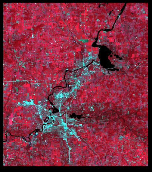 |
| Figure 1. Inquire Box subset |
 |
| Figure 2. AOI subset |
 |
| Figure 3.Original Image vs. Multiplicative Pan Sharpen |
 |
| Figure 4. Linked and Synced Google Earth View |
 |
| Figure 5. Mosaic Pro result |
 |
| Figure 6.Histogram with lower and upper change/no change thresholds |
 |
| Figure 7. Map result of Binary Change Detection |
No comments:
Post a Comment