Goals and
Background
The demand for LiDAR data grew rapidly during the early
2000s when data processing systems and IT architecture were improved to be able
to handle the terabytes of data produced by LiDAR scanners. Previous to this
time photogrammetry was used to process radar images, but this method only
produced what the scanners could “see”. Lidar scanners are able to “see”
through forested areas and are capable of gathering data about the surface
below the forest (Schukman & Renslow, 2014) . As LiDAR technology
continues to improve, the demand for its data as well as careers in the field
also continue to grow. This lab aims to provide fundamental knowledge about
LiDAR data structure and processing through specific activities involving the
processing and retrieval of surface and terrain models as well as the
processing and creation of intensity image and other derivative products from
point cloud. The files used in this lab will be in LAS format.
Methods
Part 1
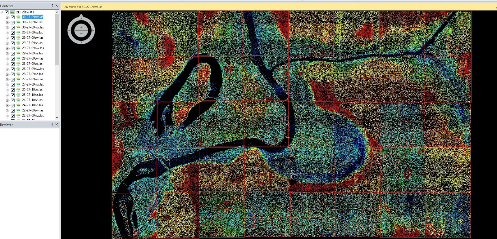
In the first part of this lab, all LAS files are displayed
together in ERDAS Imagine to visualize the point clouds as a whole image (figure 1). The LAS dataset opened in ERDAS is not
projected, however it is still possible to verify each tile`s location within
the study area. To do this a file containing quarter sections of Eau Claire
country is opened in ArcMap and the labels changed to correspond with the
individual LAS file names in ERDAS. By selecting a quarter section in ArcMap
and then selecting the same one in ERDAS, the location of each tile can be
visualized within the study area.
Part 2
This section of the lab introduces a hypothetical scenario
in which you are a GIS manager who needs to perform a quality check of LiDAR
point cloud data in LAS format as well as verify the current classification of
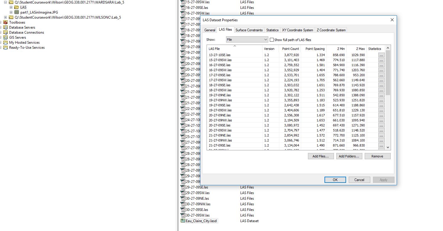
the Lidar. To begin, a dataset of all the LAS files is created using Arc
Catalog (figure 2) and the statistics for the
dataset populated using the statistics tab in the dataset properties. Most
older Lidar datasets do not have a coordinate system defined, as was the case
for this set. The coordinate system information for the point clouds can be
found in the metadata (figure 3) and then
defined under the corresponding X, Y and Z coordinate system tabs in the
dataset properties window. Now that the dataset has been appropriately
configured it can be brought into ArcMap and visualized as point cloud in 2D
and 3D. A shapefile corresponding to the area encompassing the LAS file can
also be brought into ArcMap to verify the projection was set correctly. Even
though the dataset is spatially located correctly, the identify tool will
reveal that each individual file does not have a coordinate system since this
was applied to the dataset as a whole. The point cloud can now be visualized by
activating that LAS Dataset tool bar and zooming in to 2 tiles or closer. The
point clouds can be visualized by elevation, aspect, slope, and contour. It is important to note that to view the
elevation points the number of classes in symbology needs to be changed from 9
to 8. Another method to enhance visualization for a specific purpose is to
change the filter settings, both classifications and returns can be
manipulated. For example, when the contour surface is displayed with all
returns and all classifications it is quite excessive and difficult to read. By
choosing to only display ground contours, the contour lines of the Earth`s
surface becomes much easier to interpret (figure 4).
When the dataset is displayed as points, they represent the first returns of
the laser pulse and do not have a classification, but the profile and 3D profile
view tools can be used to create an accurate depiction of small features within
the image (figure 5).
Part 3
In this section digital surface models (DSM) and digital
terrain models (DTM) will be derived from the point clouds. The models are
rasters and will need to be given a spatial resolution. The spatial resolution
should not be smaller than the nominal pulse spacing (NPS), to determine this
the average NPS for the dataset should be estimated using either the list of
point spacing values in the dataset properties tab or using the point file
information tool (figure 6). With this
information you are now ready to create a DSM with first return, a DTM, and Hillshades
of each. Since there will be numerous outputs, the current workspace should be
set to where these will be saved so this location does not have to be re-set
for each output. The LAS Dataset to Raster tool is used to create the DSM and
DTM from points elevation with the filter set to first return and ground
respectively. Each of these outputs can be enhanced by developing a hillshade,
this is done using the 3D analyst tool called Hillshade. The output of the
hillshade from the first return DMS adds a 3D appearance to the image (figure 7). The Effects tool bar contains a Swipe tool
that allows you to swipe aside the top layer to view another active layer underneath
it. This tool could be useful when one image is serving as an ancillary image
or to compare outputs. An image can also be created based on intensity, whose values are generated by the first returns. The LAS Dataset to Raster tool is also used
to accomplish this only the value field is changed to intensity instead of
elevation. The resulting image in ArcMap is very dark and obscure, however when
opened in ERDAS Imagine the output is much improved (figure
8).
Results
Lidar technology is a growing industry with an increasing
number of careers available in this field. One is also likely to encounter
Lidar data in many other geospatial careers and a fundamental knowledge of data
structure and processing is crucial. This lab has provided experience with various
components of Lidar data as well as tools for processing the data as needed.
 |
| Figure 2. Creating dataset of all LAS files |
 |
| Figure 1. Point clouds open in ERDAS |
 |
| Figure 3. Coordinate systems found in metadata |
 |
| Figure 4. Contours filtered to display onlyground classification |
 |
| Figure 5. A bridge displayed using profile and 3D view tools |
 |
| Figure 6. Point File Information tool to find average NPS |
 |
| Figure 7. Output of Hillshade tool applied to a DSM |
 |
| Figure 8. Intensity image displayed in ERDAS Imagine (left) and ArcMap (right) |
Sources
Claire, E. (2013). Lidar Point Cloud and Tile Index.
Price, M. (2014). Mastering ArcGIS 6th Edition.
Schukman, K., & Renslow, M. (2014). Penn State
Topographic Mapping with Lidar. Retrieved from History of Lidar
Development: https://www.e-education.psu.edu/geog481/l1_p4.html
No comments:
Post a Comment